The ideas in this article have been formalized (including derivations of all knockdown factors) in an AIAA paper and a reference implementation of all the methods has been made available as a MATLAB package called bat-perf.

Rob McDonald
San Luis Obispo, CA
January 2023
Originally published as a series of seven weekly LinkedIn articles from September 7 to October 18, 2022.
In Part 1, we identified some differences in the behavior of liquid fuels and batteries that are relevant for the conceptual design of aircraft. In my experience, many would-be electric aircraft developers do not adequately understand these differences.
In Part 2, we observed that the cell discharge rate map provides convincing evidence of at least two of our critical differences - that the energy delivered by a cell depends both on the state of discharge and the rate of discharge.
In Part 3, we introduced the cell specific energy knockdown factor and also a simple cell performance model appropriate for aircraft conceptual design and performance analysis.
In Part 4, we introduced an absolute energy reference for developing the knockdown factors. We also observed that the power a cell can deliver is limited along with other aspects of cell behavior including degradation through use and some aspects of charging.
In Part 5, we established reasons to limit the usable charge range of a cell. We also introduced a representative eVTOL mission profile to be used as an example for the rest of the series. We finished by calculating the partial discharge knockdown factor.
In Part 6, we developed two more components of the knockdown factor; one for capacity fade and another for finite discharge rate and resistance growth. We also defined the C rate and E rate for a cell.
In Part 7, we present the last two components of the knockdown factor and we bring it all together into a single measure of installed battery specific energy.
Part 1. How Well Do You Know Batteries?
It is natural for aircraft designers to try to think about batteries in the same terms as they would liquid fuel. There are tremendous differences, but contrasting them with something familiar gives us a framework for understanding.
While many of these differences receive lip service, I find that many would-be electric aircraft developers don’t really understand them. Ask yourself:
Do you?
Can you quantify all of these effects?
Did your quantitative understanding influence your conceptual design trades?
Energy Storage
Fuel is first and foremost a means for storing energy, so we’ll start by comparing fuel and batteries on that basis.
Liquid fuel:
Every pound of fuel is equally energetic.
The rate of consumption does not diminish the energy in fuel.
A fuel tank’s capacity does not diminish with use.
Energy required determines the required fuel quantity.
Every pound of fuel can be replaced at the same rate.
Batteries:
The energy contained in different parts of a cell are not equal.
When discharged rapidly, a cell will deliver less energy.
The capacity of cells degrades with use and time.
Energy required may determine the required battery size.
Charge rate varies – cells are very slow to top off.
Power Source
Though seldom a concern, the fuel flow rate is a means of providing power.
Liquid fuel:
Every pound of fuel is equally powerful.
Fuel can be consumed at almost any rate.
The power capability of fuel does not diminish with use.
Power requirements determine the size of the engine.
Fuel burning A/C perform better at end of mission.
Batteries:
The power available from different parts of a cell are not equal.
Cells can only discharge at a limited rate.
The power capability of cells degrades with use and time.
Power requirements size the motor & drive – and may size the battery.
Battery powered A/C perform worse at end of mission.
So what do you think?
I’ve been thinking about writing a series of posts to dive into this. Thoughts?
A) You aren’t a professor anymore, don’t lecture us on batteries.
B) BatteryStartup says they will get 800 Wh/kg next year. That is all I need to know.
C) I’m battery curious - tell me more.
Part 2. Beginnings
Before we can discuss, understand, and quantify the differences between batteries and liquid fuel, we need to cover some background, define some terms, and maybe even show an equation or two. Things may start basic, slow, and long - but should pick up as we go along.
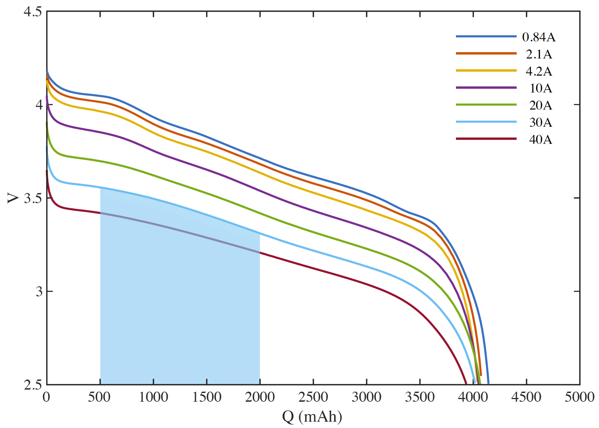
A cell discharge rate map is the fundamental chart depicting cell performance. They are commonly depicted on a manufacturer’s data sheet.
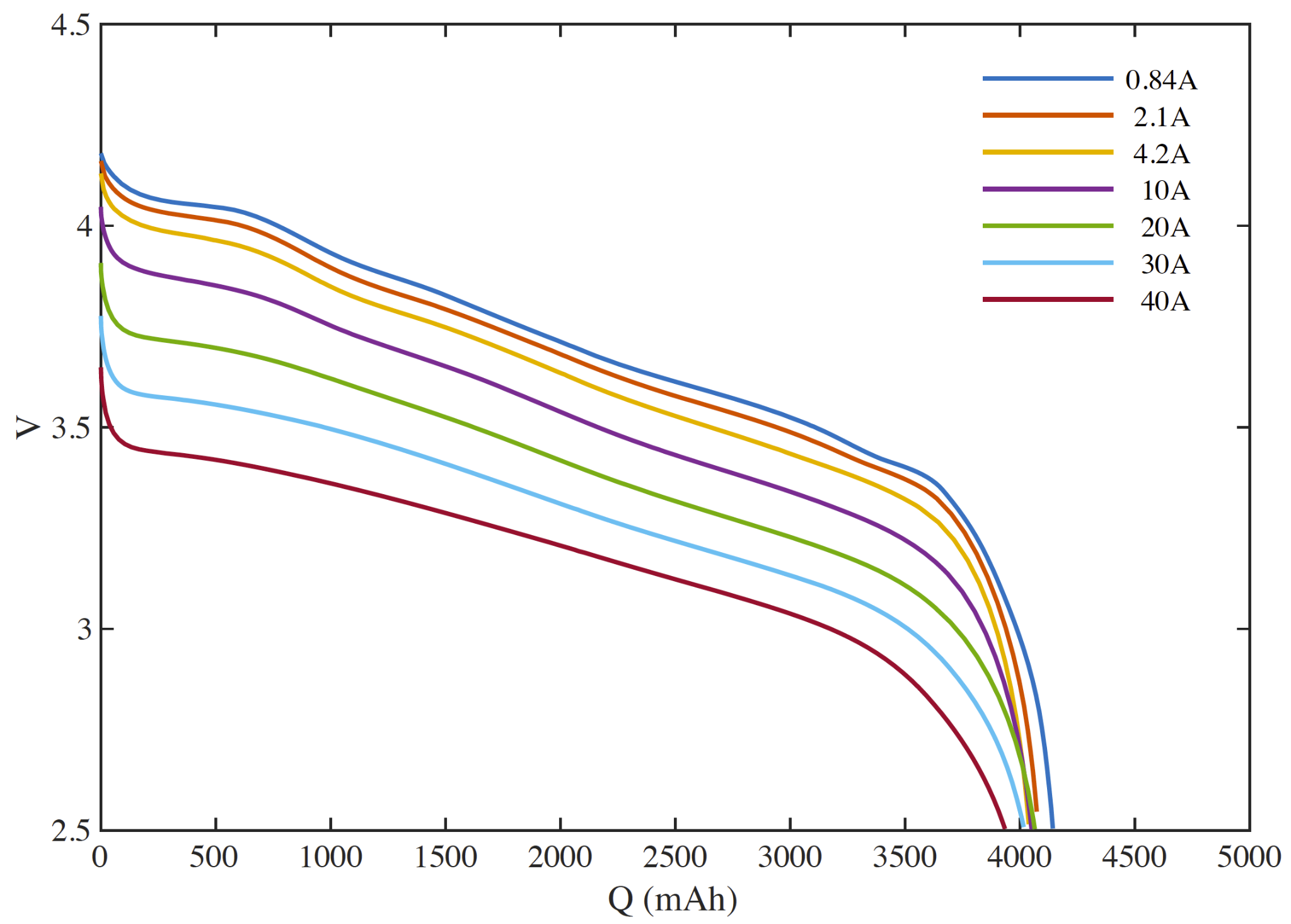
A rate map depicts the discharge voltage (vertical axis) as a function of cell capacity (horizontal axis) for different constant current discharges (each colored line).
Cell capacity is measured in charge. Here, mAh (milli-Ampere-hours), but you should be familiar with Ah, As, and Coulomb (C) – one C = 1As.
A meander: You may think it would be more natural to conceptualize cell capacity in terms of energy. Unfortunately, this doesn’t work out. Like mass, momentum, and energy, charge is a conserved quantity. We can track the flow of charge in and out of a cell – the EE’s call this ‘Coulomb counting’.
You’ll be glad to know the first law still applies – energy is conserved when charging or discharging a battery. However, some energy goes to waste heat due to the cell’s internal resistance. This ‘lost’ energy would make tracking the contents of a battery very difficult.
Of course, we do not track the contents of fuel tanks in terms of energy either. Instead we use mass/weight or perhaps volume.
The commonly used units of charge (Ah) is admittedly awkward, but analogous to using light-years to measure distance. One Ampere of current is one Coulomb per second flow of charge.
The cell depicted in our rate map is nominally a 4200 mAh cell. The horizontal axis depicts the capacity discharged from full such that the cell is full on the left and empty at the right.
At a given state of discharge (say 1000 mAh) and discharge rate (say 10 A), the voltage across the terminals will be about 3.8V. Increasing the discharge rate will cause the voltage to drop. Likewise, discharging at the same rate, but at a deeper state of discharge will also occur at a lower voltage.
The area under a discharge curve is the energy delivered during that discharge. This is depicted for a full-depth discharge at 10 A as the shaded region below.
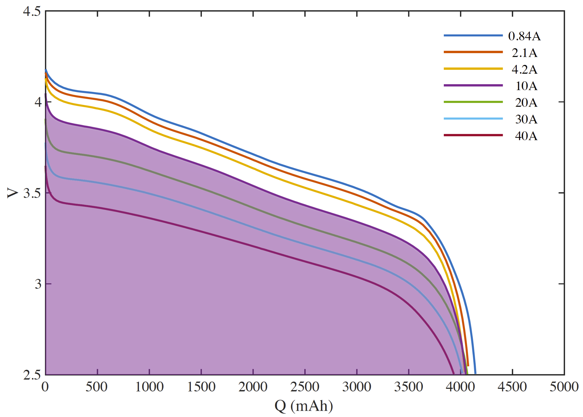
In order to zoom in on the interesting part of the chart, the vertical axis of discharge rate maps usually does not go to zero, so be careful about visually comparing areas under the curves - there is often more area off the chart than on.
We can now see that a 10A discharge of 500 mAh from a relatively full cell will provide more energy than the same discharge from a relatively empty cell.
Putting this in terms of liquid fuel (without proof or further discussion), we realize that the first pound of fuel in a tank contains the same energy as the last pound of fuel in the tank.
We are ready to observe the first of our key differences between liquid fuel and batteries.
- The energy contained in different parts of a cell are not equal.
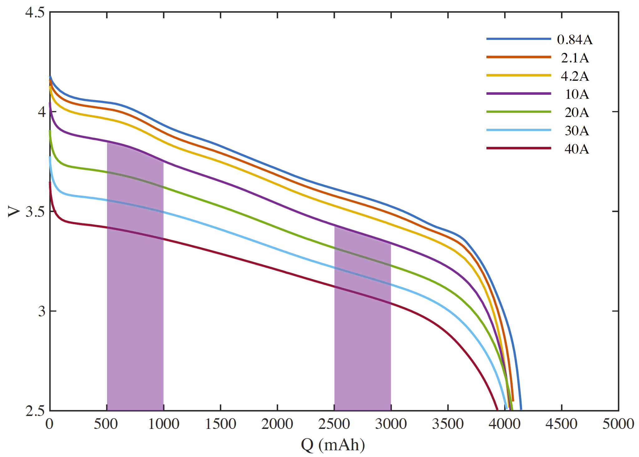
We can also see that a 1500 mAh discharge starting at the same depth of discharge will provide more energy if performed at a lower discharge rate (say 10A vs. 30A) (the ’lost’ energy goes to waste heat due to the cell’s internal resistance). The higher rate discharge will also take 1/3 the time.
In terms of liquid fuel, we understand that a pound of fuel contains the same energy no matter how quickly we pump it through the lines.
We now observe the second of our key differences between liquid fuel and batteries.
- When discharged rapidly, a cell will deliver less energy.
The discharge rate map has more secrets to reveal, but that is enough to get us started. Become comfortable with rate maps - they’ll be back.
How am I doing?
Thanks to everyone who reacted to my first post - while perhaps smaller in number than hoped, the reaction was entirely positive. So begins the journey.
Please let me know how I’m doing.
Part 3. Bottom Line
This is one of those stories that requires a lot of background. Here we’ll make one more big push to get us ready for the main event.
Undoubtedly, the critical technology metric for the application of batteries to aircraft primary propulsion is the specific energy - the energy per mass of a battery.
(Without any offense to power, we will briefly focus our discussion on matters of energy. Don’t worry, power’s critical role in this story will come.)
Manufacturer’s Cell Specific Energy
Cell manufacturers quote the cell specific energy under defined idealized laboratory conditions - the energy provided by a cell when discharged in a particular way divided by the cell mass.
$$e_{\mathrm{mfg}}=\frac{E_{S,c}}{m_{c}}$$The manufacturer’s cell rated energy is typically obtained from a full-depth discharge at constant current. For ’energy cells’ this discharge is relatively slow (say 0.2C), and for ‘power cells’, this discharge is substantially faster (say 1C).
Effective Battery Specific Energy
As previously discussed, the energy delivered by a battery depends on both the state of discharge (when the discharge occurs) and the rate of discharge (how the discharge occurs). I.e. the energy delivered depends on the details of the cell discharge profile.
We will define the effective specific energy of a battery in the terms most relevant to aircraft design - the energy required for an aircraft to fly the critical sizing mission divided by the mass of the battery pack.
$$e=\frac{E}{m_{b}}$$Knockdown Factor
We will define a cell energy knockdown factor to account for the differences between the manufacturer’s specific energy and the effective specific energy.
$$e=k\,e_{\text{mfg}}$$Much of our coming discussion will focus on understanding and quantifying this knockdown factor for each of the identified differences between liquid fuels and batteries. Spoiler alert - stark realities await.
Modeling a Cell’s Behavior
A cell’s performance can be modeled with a simple equivalent circuit consisting of a voltage source and a resistor in series.
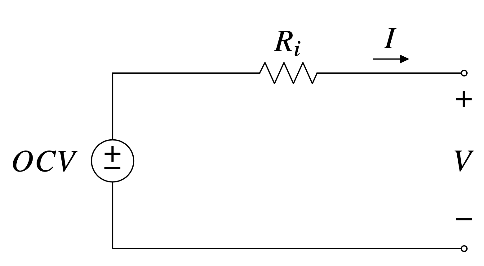
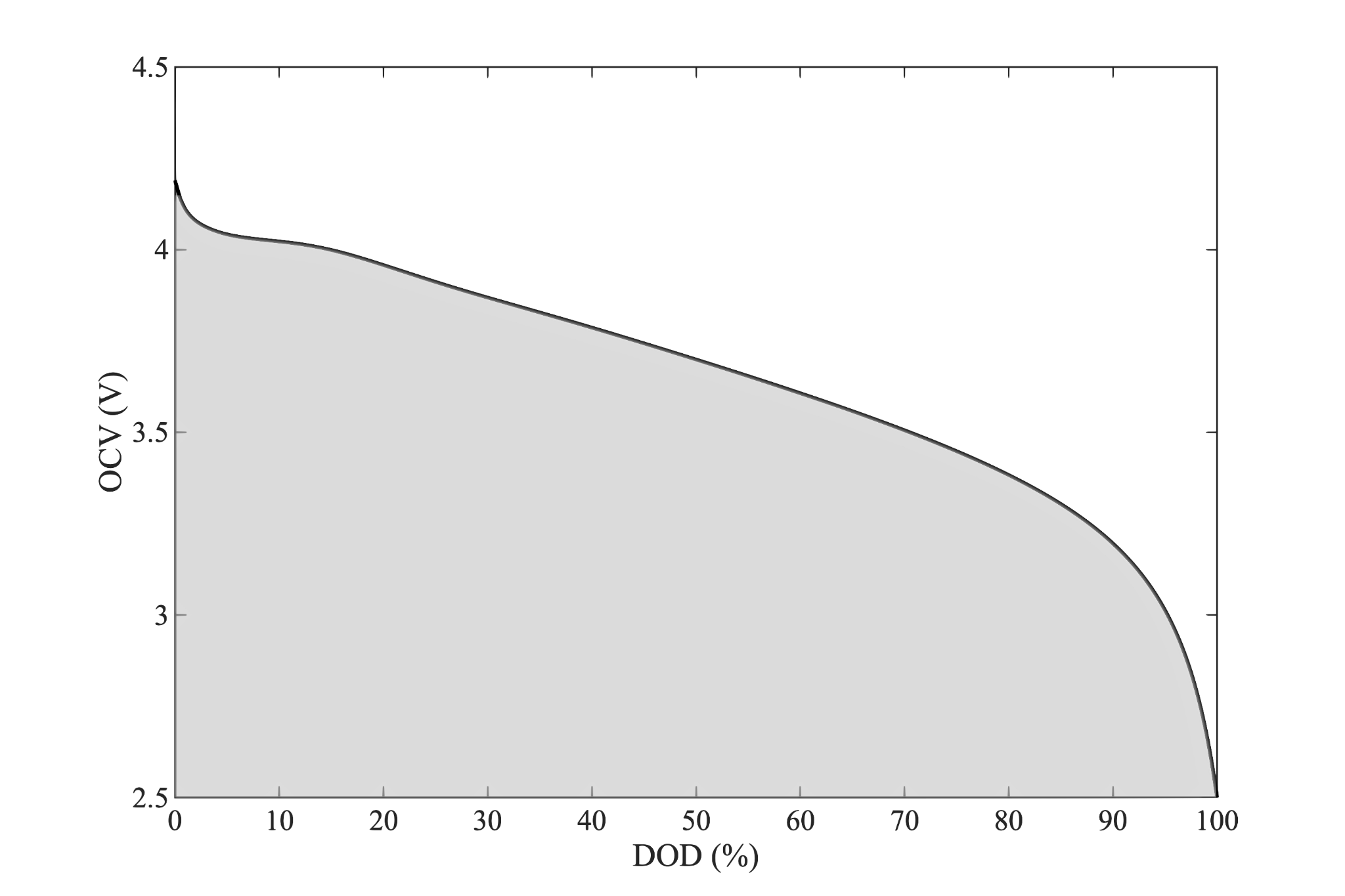
The potential across the voltage source is the cell’s open circuit voltage and the resistance is the cell’s internal resistance. Both the $OCV$ and the $R_i$ are functions of the cell depth of discharge - they depend on where you are in a cell’s discharge.
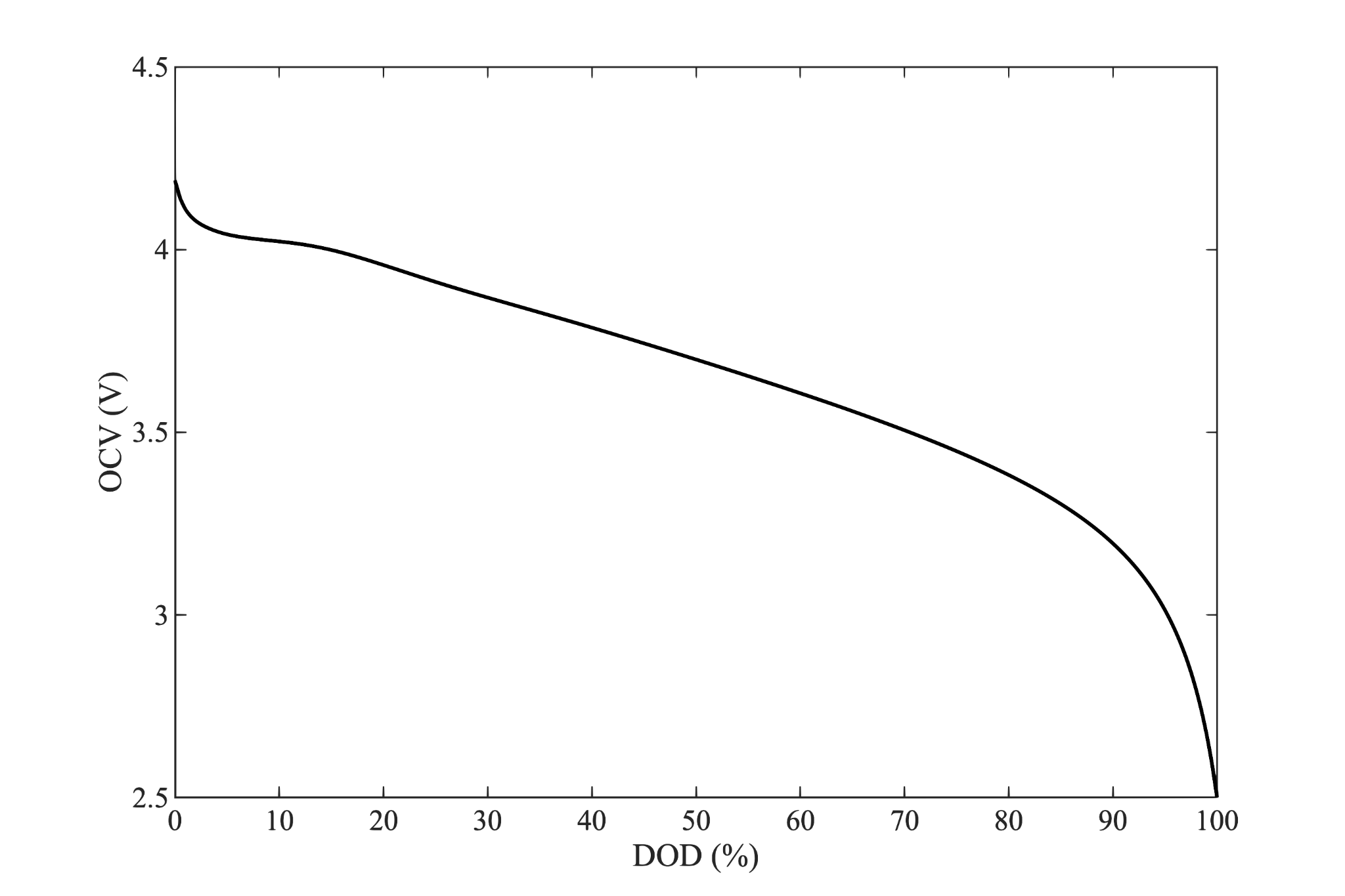
(Note that here we use the depth of discharge ($x$) as a fraction of the rated cell capacity ($Q$).)
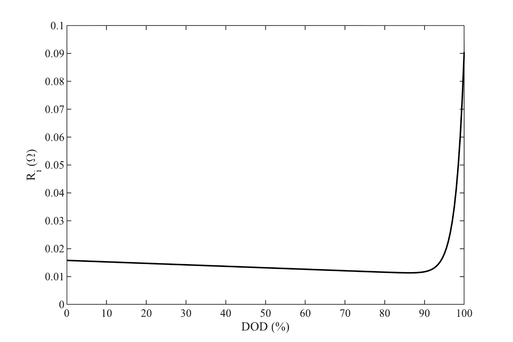
We will require $OCV$ and $R_i$ curves like those shown above. These may be provided by the cell manufacturer or they can be reverse engineered from a typical discharge rate map. Although there are theoretical means of predicting these curves, they are almost always empirically derived in practice. The functional form of these curves is irrelevant to our purposes, linear interpolation or functional fits to data are acceptable.
The equation for the cell terminal voltage allows us to calculate the cell voltage given the depth of discharge and the rate of discharge. This provides us with an equation of state for the cell.
$$V\left(x,I\right)=OCV\left(x\right)-R_{i}\left(x\right)\,I$$(Many cell modeling resources will expend great effort including capacitance in the form of one or more RC circuits in the cell model. This adds an additional time response to the cell’s behavior. Fortunately, for purposes of conceptual aircraft design, we can limit ourselves to the cell’s steady state resistance. During conceptual design, an aircraft’s power draw is typically treated as a series of constant power segments. The time spent at each power level is long compared to the time response of the cell.)
In addition to predicting the cell’s terminal voltage at any instant in time, we need to track how the cell’s state of charge changes with time. For this, we write a simple statement for the conservation of charge.
$$\frac{\mathrm{d}x}{\mathrm{d}t}=\frac{I}{Q}$$Given these equations and models, a little bit of algebraic manipulation and some integration is all that we will need to model cell behavior for aircraft design.
(When the time comes, we will slightly modify these models to account for cell ageing.)
Checking In
If you made it this far, make a comment and let me know what you think.
Although I initially promised a ‘deep dive’, I still feel the need to keep these articles pretty high level. Consequently, I don’t plan on actually showing the algebraic manipulations of the terminal voltage equation or the integration of the conservation of charge. I’m going to trust that if you are sufficiently motivated, you can figure that out. Reach out if more detail is required.
Part 4. An Absolute Reference
The cell specific energy knockdown factor introduced in Part 3 relates the manufacturer’s rated specific energy to the effective specific energy for an aircraft. While this is the ‘right’ metric (most useful to an aircraft designer), it would prove cumbersome to calculate directly.
Instead, we consider the limit of the energy discharged from a cell as the rate approaches zero. Such a zero current discharge would take infinite time, but it would also suffer no losses to internal resistance. We often think of lossless, infinite-time processes as reversible - we will use that term here.
The reversible cell energy is the true energy stored in the cell. When discharged at a finite rate, some of that energy is released as useful electricity and the rest is lost as waste heat.
Just as the energy for a given discharge is the area under the voltage vs capacity curve, the cell reversible energy is the area under the $OCV$ curve.
Power is Limited
The instantaneous power discharged from a cell may be computed by multiplying the terminal voltage equation by the discharge current.
$$P\left(x,I\right)=OCV\left(x\right)\,I-R_{i}\left(x\right)\,I^{2}$$The maximum power a cell can discharge can be found through the familiar calculus routine. 1) Take the derivative of the power equation with respect to current. 2) Set that equal to zero. 3) Solve for the current at maximum power. 4) Substitute back into the power equation to determine the maximum discharge power given here.
$$P_{max}\left(x\right)=\frac{\left(OCV\left(x\right)\right)^{2}}{4\,R_{i}\left(x\right)}$$This power level itself is not particularly useful - it is unreasonably high and other bad things will likely happen before reaching it. In particular, at this power the cell instantaneous efficiency is 50% - half of the cell’s energy is going to waste heat.
The first important observation is that a limit on power exists - demonstrating another one of our bullets from Part 1: Cells can only discharge at a limited rate.
The second important observation is that this power limit is a function of the depth of discharge - another bullet: The power available from different parts of a cell are not equal.
The third important observation is that the internal resistance of a cell is intimately linked to the maximum discharge power. Double the internal resistance and the maximum power is cut in half!
Similar procedures may be carried out to determine other limits on the cell discharge power. The figure below compares four possible limits on cell power discharge. The magnitudes of these limits are not important - the constraining quantity has been chosen to bring each corresponding power limit to roughly the same value for comparison. The absolute power limit derived above is the solid line on this graph.
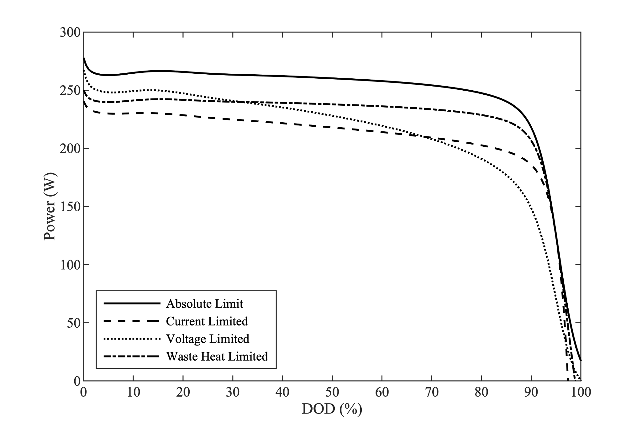
Years ago in EE lab, I learned that everything is a fuse if you put enough current across it. There will be a maximum current limit associated with the cell and the pack. Perhaps it will be determined by the fuseable link connecting each cell. Perhaps it will be determined by a module or pack fuse. Perhaps it will be determined by the gauge of wire connecting the pack to the bus bars - or the dimensions of the bus bar itself. There will be a current limit. It will be shaped like the dashed line in the figure above.
Similarly, there will be a minimum voltage limit somewhere in the system. Perhaps it will be determined by the cell cutoff voltage. Perhaps it will be determined by a power electronics brownout condition where it becomes impossible to command full RPM. A cell minimum voltage limit will look like the dotted line in the figure above.
There may be other limits. Perhaps a maximum waste heat limit imposed by the battery pack cooling system. A waste heat limit will look like the dash-dot line in the figure above.
We again observe that each of these power limits is a function of the depth of discharge of the cell. In particular, we observe that the power limits tend to decrease with depth of discharge. I.e. the battery’s limit discharge power is less at the end of a mission than at the start - another bullet from Part 1: Battery powered A/C perform worse at end of mission.
A battery pack for an aircraft with a large power requirement at the end of the mission will likely be sized by power instead of energy - one more bullet: Power requirements may size the battery.
The most common example of such a requirement is an eVTOL vehicle landing at the end of the mission. However, eCTOL vehicles executing a go-around at the end of a mission may also provide a sizing power requirement.
We do not have scope to demonstrate it, but like the absolute power limit, each of the power limits discussed here is strongly linked to cell internal resistance. Increasing internal resistance will reduce the maximum power capability of a cell or pack.
Finally, we observe that these lines are not parallel; depending on the details of the values of each constraint, these lines can and will cross. I.e. which factor is limiting will change throughout the discharge.
You may think you can design a power system such that only one power limit is ever active. Or such that no power limit is ever critical. Such a system will never be optimal; it is guaranteed to carry extra mass to provide that margin.
Cell Ageing
Cell performance degrades. Anyone who has worked with an old laptop or cell phone has experienced this. Cell degradation is caused by tiny amounts of damage done to the cell. This damage occurs every time we charge or discharge a cell. It can even occur if we just leave a cell sitting on a shelf.
There are two primary aspects of cell degradation. The cell capacity will reduce; this is called capacity fade. At the same time, the cell internal resistance will increase; this is called resistance growth or power fade (recall the importance of resistance to power).
Thus we have two more Part 1 bullets: The capacity of cells degrades with use and time. & The power capability of cells degrades with use and time.
There are two main sources of cell degradation. Calendar ageing is damage done to a cell over long periods of time independent of charging and discharging. Calendar ageing is most rapid in a cell that is kept fully charged at all times. We are typically less concerned with calendar ageing for aircraft that we hope to operate at high tempo.
Cycling ageing is damage done to a cell during any charge or discharge. The rate of cycling damage depends on the rate of charge or discharge and also on which portion of a cell is cycled.
In the data below, we observe that capacity fade and resistance growth are greatest for the cells cycled at the top of charge (gold and purple) and the bottom of charge (blue). The least damage occurs for the cells cycled in the middle of the discharge range (green, red, and cyan).

J. Schmalstieg, S. Käbitz, M. Ecker and D. U. Sauer, ‘From accelerated aging tests to a lifetime prediction model: Analyzing lithium-ion batteries,’ 2013 World Electric Vehicle Symposium and Exhibition (EVS27), 2013
Theoretically, an aircraft whose battery is sized without consideration of ageing will only be able to execute its design mission once. During that singular mission, some damage to the cell will occur - reducing the capacity and increasing the internal resistance - reducing the range or endurance of the aircraft and its peak power capability.
Any aircraft destined for practical operation must consider ageing in the pack design. It may be reasonable to ignore ageing for flight concept demonstrators, but beware this reality.
Charging
Like cell ageing, charging is a complex subject that we will not attempt to do proper justice. Any cell that is discharged will need to be charged. Charging is typically performed with a CCCV process (constant current, constant voltage).
During the CC phase of a charge, a cell is charged at constant current. A cell’s state of charge can rapidly increase during the CC phase. The CC phase ends when the terminal voltage reaches some charge voltage (the maximum voltage limit for the cell). At that point, the charge cycle changes to CV - the charge voltage is maintained until the current drops below some tiny threshold and the cell is declared full.
During the CV phase of a charge, the charge current is constantly decreasing. At decreasing current, it takes increasing time to increase the charge of the battery. This is an asymptotic process - it takes infinite time to fully charge a cell to zero charge current.
I don’t know about you, but asymptotic processes don’t seem like a good idea for concepts intended for high tempo operations.
This gets us to our final battery bullet from Part 1: Charge rate varies – cells are very slow to top off.
Progress
I know I keep saying that we’re nearly through all the background - but this time it is true. We’ve justified every single one of our battery bullets from Part 1. You should have an understanding of why each one is true and some intuition about the complexities of cell behavior.
Of course we aren’t done yet. I promised to show how to quantify these effects - and we will do so by computing each one as a contribution to the overall cell energy density knockdown factor. The pieces are in place, we’re just about ready to start knocking down the knockdown factors.
Part 5. Charge Limits
In Part 4 of this series, we discussed several cell characteristics that may have seemed unrelated - power limits, cell degradation due to cycling, and charging. In fact, these characteristics conspire to limit how much of a cell’s charge is available for use.
Although a cell has a certain rated capacity (typically given in mAh, but we will work in terms of percent of that capacity), for the purposes of conceptual design sizing, some of that capacity is unavailable to us.
Some of that unavailable charge is the first few percent discharged from a full battery; we call that region the Top of Charge. There is also some unavailable charge that would be the last few percent discharged from a battery; we call that region the Bottom of Charge.
Some of these limits are more fungible than others. We will start with the firm and move towards the flexible.
Power Limits for Bottom of Charge
In Part 4, we discussed the limits on power that can be discharged from a cell (figure repeated here). We identified that there are at least four causes of these limits (absolute, current, voltage, waste heat) and that these limits vary with depth of discharge.
Thinking in terms of an aircraft, there will be some minimum power required of the cells late in the mission. While this may simply be to maintain cruise flight, it likely involves a higher power requirement such as aborting a landing or arresting the descent in a vertical landing.
If that requirement worked out to 175W per cell, then the power limit chart from Part 4 tells us that we can not go past 85% DOD and achieve the required power. If we were to demand more than 175W at 85% - or 175W beyond 85%, then our bus voltage would drop below the cutoff voltage and our power electronics would not be able to command the speed and power required for this mission phase.
Unfortunately, this means that 15% of our battery is dead weight. We are forced to carry it around with us, but we can not get ourselves into a situation where we use it.
Cell Ageing for Top and Bottom of Charge
In Part 4, we also discussed the damage that accrues to a cell from every use. We observed that damage occurs faster for cells discharged at the top and bottom of charge (figure repeated here).
J. Schmalstieg, S. Käbitz, M. Ecker and D. U. Sauer, ‘From accelerated aging tests to a lifetime prediction model: Analyzing lithium-ion batteries,’ 2013 World Electric Vehicle Symposium and Exhibition (EVS27), 2013
The aircraft designer must choose the conditions that define the battery end of life. This will correspond to a certain amount of capacity fade (say 15%) and a certain amount of resistance growth (say 20%). This capacity fade and resistance growth will factor into the cell knockdown factors at a later time. In addition, the designer must consider how many cycles the cells must survive for the economic case to close. For example, do you need to hit 3000 cycles, or can you afford to replace packs at 1000 cycles?
For this cell to reach EOL at 3000 cycles, we will need to restrict our cycles to be between 20% and 80% SOC (note that SOC=100%-DOD). I.e. we need to avoid the first 20% and last 20% of the cell to maximize life.
The bottom of charge restriction for life is fortunately not very severe. First, it typically substantially overlaps with the limit already imposed by power. Second, most aircraft sizing missions require some sort of reserve - a mission segment that must be able to be flown, but that is not flown frequently. Placing this reserve in a portion of a cell with rapid damage accrual may be acceptable because the reserve is not used frequently. Of course, we still expect the high power draw requirement to apply at the end of any reserve mission.
Conversely, the top of charge restriction for life is painful. Maximizing cell life requires that you avoid topping off your pack and instead size with the assumption that you start missions with a pack that is only 80 to 90% full.
Obviously, cell ageing presents complex tradeoffs for the designer. What defines cell end of life? How many cycles to replacement? How do we operate our packs to maximize life?
Rapid Charge for Top of Charge
As discussed in Part 4, the constant voltage (CV) portion of a charge cycle is very slow to top off a cell. For some systems and conops, this will pose no obstacle. However, for missions and conops where many sorties, quick turnaround, fast tempo, and rapid charging are important, you will want to avoid or limit time spent charging in this mode.
One interesting perspective is to consider the energy added during charge as incremental miles of range - and then to consider how quickly each mile is added (miles of range per minute of charge).
Like ageing, charging rate is a part of more complex trades, but it can contribute to a restriction on the usable charge range for a pack.
Representative eVTOL Mission
We will introduce an extremely simple eVTOL mission profile along with some other assumptions that will provide an example case for the rest of this series.

This mission includes a primary segment followed by a reserve mission requiring a divert. Each segment is made up of a takeoff, cruise, and landing segment. Each segment is specified in terms of time and power level as given below.
| Segment | Duration | Power |
|---|---|---|
| (m) | (hp) | |
| Takeoff Hover | 1 | 500 |
| Cruise | 20 | 50 |
| Landing Hover | 1 | 500 |
| Reject | 1 | 500 |
| Divert | 5 | 50 |
| Landing Hover | 1 | 500 |
The battery will reach end of life when it reaches 10% capacity fade or 20% resistance growth.
The cell usable charge will be restricted to avoid 10% at top of charge and 15% at bottom of charge.
Partial Discharge Knockdown
We are finally ready to calculate our first cell energy knockdown factor. The partial discharge knockdown defined as the usable energy divided by the total cell energy. Recall that the total cell energy is the area under the $OCV$ curve (the grey line in the figure below). The pink regions indicate the un-usable discharge - leaving the usable energy as the white space between them.

For mental calculations, we can assume that each portion of charge contains equal energy, allowing us to approximate the partial energy knockdown as the usable charge fraction.
$$k_{e,DOD}\approx BOC-TOC$$$$k_{e,DOD}\approx0.85-0.1=\,0.75$$Of course, the $OCV$ is not constant and we have gone to lengths to understand that different portions of a cell’s charge store different energy. If we calculate the running total energy available in a cell (normalized by the total), we would get a curve like this:

This curve starts out steeper than the equal distribution curve because the top of charge contains more energy per charge than the cell average.
At 10% DOD, we are at perhaps 11% energy, and at 85% DOD, we are at perhaps 87% energy - we subtract these and adjust our estimate of the partial discharge knockdown to 0.76.
This figure is hard to read with great precision. So I have subtracted the equal distribution curve from the running total to arrive at a figure that magnifies the quantities of interest.

Using this figure, we can calculate the partial discharge knockdown factor.
$$\begin{matrix} {k_{e,DOD}=}&{BOC+D\left(BOC\right)}\\ &{-\left(TOC+D\left(TOC\right)\right)} \end{matrix}$$$$\begin{matrix} {k_{e,DOD}=}&{0.85+0.024}\\ &{-\left(0.1+0.011\right)}\\ {\,\,\,\,\,\,\,\,\,\,\,\,\,\,\,\,\,=}&{0.763}\\ \end{matrix}$$While there are several more knockdown factors (more bad news) yet to come, this one is usually the hardest pill to swallow (this was the worst of it).
Still With Me?
It has taken a while to get to this point, but we’ve discussed the cell behaviors that make them a challenge for aircraft design. We introduced the knockdown factor as our primary metric of interest. Now we’re starting to quantify those effects. Things are going to move fast from here on.
If you made it this far, leave me a note and tell me what you think.
If you find this thought provoking, hit share and add your thought as a comment.
Part 6. Roadmap
In Part 3, we introduced the idea of a cell specific energy knockdown factor that captures a variety of phenomena relevant for battery performance and aircraft design. We are working our way through each of these phenomena, calculating how each one contributes to the overall knockdown factor. In Part 5, we developed the cell partial discharge knockdown factor.
Capacity Fade Knockdown
When we defined our representative mission in Part 5, we defined battery end of life as occurring when the cell reaches 10% capacity fade or 20% resistance growth. In our analysis, we will assume the cell has reached both of those limits at EOL.
The cell capacity fade knockdown factor is too simple to be called a derivation, it is simply the fraction of cell capacity remaining at end of life. For our case, this is 90%.
$$k_{Q}=0.9$$One-Hour Discharge Rates
Battery people often work and communicate in terms of a discharge current scaled to the size of a given cell. They define the current required to fully discharge a cell (at constant current) in one hour as the 1C current for that cell. If you know a cell’s capacity, then it is trivial to calculate that cell’s 1C rate - a 4200 mAh cell has a 1C discharge rate of 4.2A.
A similar idea can be applied to a constant power discharge. We will define the power required to fully discharge a cell (at constant power) in one hour as the 1E power for that cell. Unfortunately, calculating the 1E power is not trivial - it requires numerically solving over the discharge integral. However, since aircraft fly at power settings (not current settings), it is a more useful quantity.
We will also need to know the E rate required for a sized battery to complete a given mission. Of course, this whole series is about sizing a battery - so if we need to know the battery size to calculate the battery size, things are going to get iterative.
As an initial guess, we will do some back of the envelope calculations. First, we need to know the total energy required to fly the example mission. We simply sum the products of the time and powers for each segment. Don’t worry about the horrible units, they will cancel out in a moment. Our mission requires 3250 hp-m of energy.
| Segment | Duration | Power | Energy | Power |
|---|---|---|---|---|
| (m) | (hp) | (hp-m) | (E-Rate) | |
| Takeoff Hover | 1 | 500 | 500 | 6.23 |
| Cruise | 20 | 50 | 1000 | 0.623 |
| Landing Hover | 1 | 500 | 500 | 6.23 |
| Reject | 1 | 500 | 500 | 6.23 |
| Divert | 5 | 50 | 250 | 0.623 |
| Landing Hover | 1 | 500 | 500 | 6.23 |
| Total | 3250 |
Next, we need to make some adjustments for the size of the cell. That is the crux of these knockdown factors (complicating the iterative process), but we can at least take some first steps. We will use our crude estimate from Part 5 of the partial discharge knockdown factor as well as our capacity fade knockdown factor.
$$P_{1E}\approx\frac{1}{\,\left(0.75\right)\,\left(0.9\right)}\frac{3250}{60}$$To obtain our estimate of the 1E power required of our sized pack, we divide the total energy requirement by these adjustment factors and also by 60 minutes (to establish the one-hour rate). The 1E power for this vehicle is about 80.25 hp. Unsurprisingly, the cruise occurs at an E rate substantially less than 1.0 (0.623).
Finite Rate Knockdown
In Part 2, we recognized the area under the discharge curve on voltage vs. capacity axes as the useful energy provided by the cell during that discharge. In Part 4, we identified the area under the $OCV$ curve as the reversible energy stored in a cell.
These are both total (integral) measures - the total energy discharged and the total energy available. If we take their ratio, we would obtain some measure of the cell efficiency for a discharge. This would be a knockdown factor that accounts for the effects of a finite rate discharge.

Here the black discharge curve is the discharge profile for our example vehicle introduced in Part 5. The discharge energy required to complete the mission is the area in grey. The area under the corresponding portion of the $OCV$ curve includes the pink and grey areas.
While we can numerically integrate a discharge profile to arrive at the finite rate knockdown factor, that does not provide us with much insight into what is happening during different mission segments and their relative impact on battery performance.
Cell Instantaneous Efficiency
We can extend this idea to a single instant during a discharge. The arrows indicate the terminal voltage and the $OCV$ during the second high power discharge of the mission (the nominal landing hover). The ratio of these voltages is the cell discharge efficiency at that instant of the mission.
$$\eta_{i}=\frac{V}{OCV}$$For aircraft performance and sizing, we are usually concerned with discharge at a certain power level. We can put the instantaneous efficiency in terms of a desired power draw.
$$\eta_{i}=\frac{1}{2}+{\sqrt{\frac{1}{4}-\frac{R_{i}\,P}{OCV^{2}}}}$$This equation makes clear the importance of low internal resistance for efficient discharge at high power.
Finite Rate and Resistance
We will make two modifications to this equation with the goal of simplifying and isolating things that change during a mission or the life of a battery from things that are constant for a given cell. First, we will replace the cell internal resistance with a resistance growth factor applied to the cell internal resistance of a brand new cell. Second, we will replace the discharge power with the discharge E rate with the power for a 1E discharge.
$$\eta_{i}=\frac{1}{2}+{\sqrt{\frac{1}{4}-\frac{k_{R}\,E_{rate}\,R_{i,0}\,P_{1E}}{OCV^{2}}}}$$Of course, the BOL cell internal resistance ($R_{i,0}$) and $OCV$ are functions of depth of discharge, but we have dropped the $f(x)$ notation for clarity.
We observe that the resistance growth factor ($k_R$) and the discharge E rate appear as a product - if we treat them as a composite quantity, the effect of a 20% increase in $k_R$ is indistinguishable from the effect of a 20% increase in E rate.
Recall that our mission profile and battery assumptions from Part 5 defined battery end of life as occurring when the cell resistance grew by 20% - i.e. $k_R=1.2$. This equation demonstrates that an EOL cell discharging at 5E will achieve the same instantaneous efficiency as a BOL cell discharging at 6E.
We can generate a plot of cell instantaneous efficiency parameterized by the composite quantity ($k_R\,E_{rate}$), shown in the black lines below.
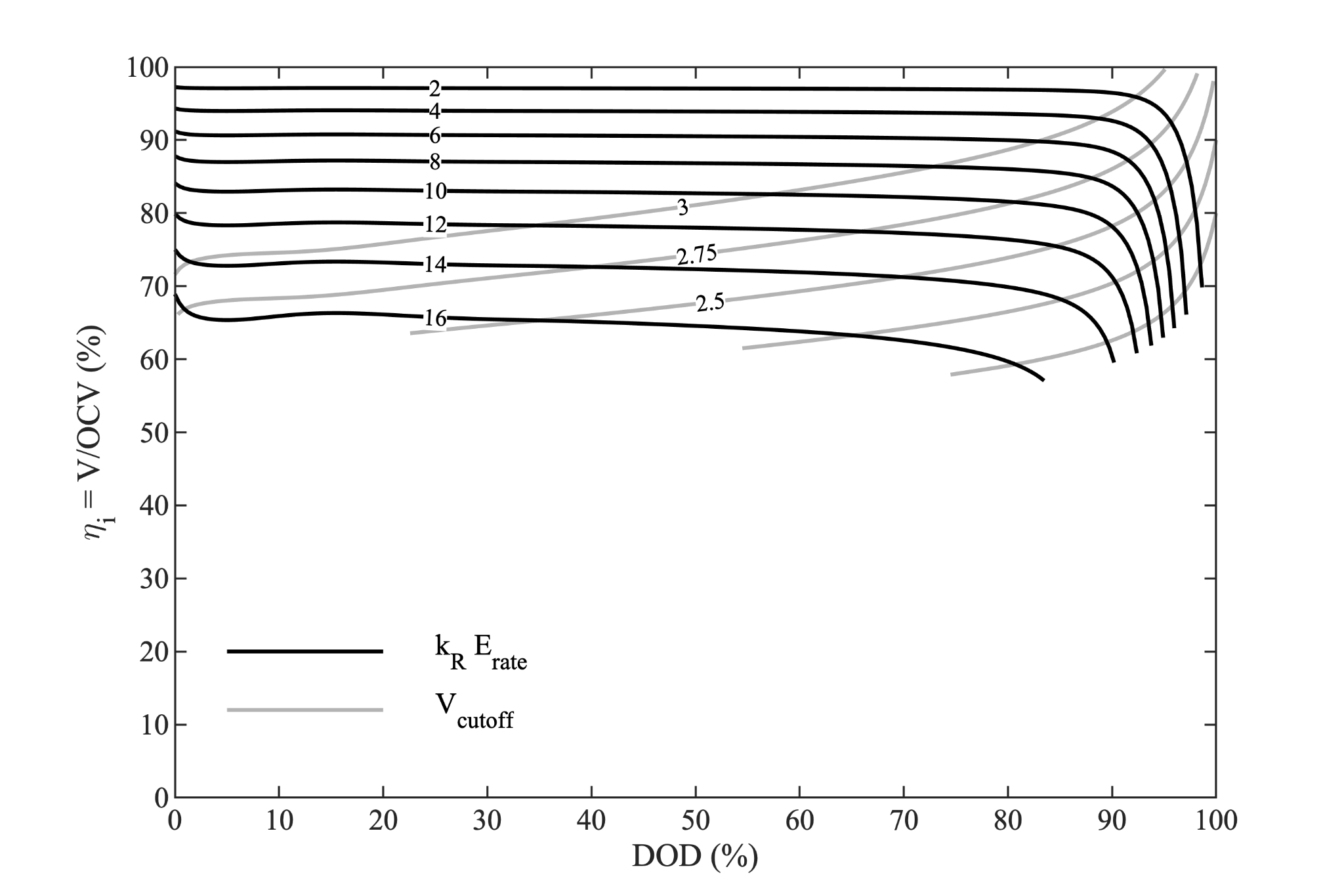
In this figure, additional grey lines are included to illustrate the effect of the cell cutoff voltage - the minimum voltage power limit. Other power limits could be plotted in similar fashion.
Although the black lines in this figure appear remarkably flat over a wide range of DOD, that is not a general result. It is just a lucky coincidence for this cell. Alternatively, we can plot this same information parameterized by depth of discharge, as a function of rate.

The fact that the curves were remarkably flat in the prior figure leads to the lines for different depth of discharge nearly collapsing in this figure.
To calculate the instantaneous efficiency for each mission segment at the battery end of life, we multiply the segment E rate by the EOL resistance growth factor. For cruise, this gives $k_R\, E_rate=1.2\*0.623=0.7476$; and for hover, 7.476.
Using the above chart, we see that instantaneous cell efficiency during cruise is about 99% while during hover it is about 88%. We can add this information to our mission profile table.
| Segment | Duration | Power | Energy | Power | ηi |
|---|---|---|---|---|---|
| (m) | (hp) | (hp-m) | (E-Rate) | ||
| Takeoff Hover | 1 | 500 | 500 | 6.23 | 0.886 |
| Cruise | 20 | 50 | 1000 | 0.623 | 0.990 |
| Landing Hover | 1 | 500 | 500 | 6.23 | 0.884 |
| Reject | 1 | 500 | 500 | 6.23 | 0.882 |
| Divert | 5 | 50 | 250 | 0.623 | 0.989 |
| Landing Hover | 1 | 500 | 500 | 6.23 | 0.877 |
To obtain the integrated knockdown factor discussed earlier in this article, we would ideally integrate the instantaneous efficiency throughout the mission. Alternatively, we can compute an average efficiency weighted by the energy expended in each mission segment according to the following equation.
$$k_{e,FR\&R}=\frac{\sum_{i}^{n}E_{i}}{\sum_{i}^{n}\frac{E_{i}}{\eta_{i}}}$$This gives us the cell energy knockdown factor for the effects of both finite rate discharge and resistance growth. Running the numbers yields 0.92 for this value.
$$k_{e,FR\&R}=0.92$$Light at the End of the Tunnel
If you’ve made it this far, congratulations. You’re almost done. We now know how to calculate three contributions to the cell energy knockdown factor (covering four physical phenomena). Next week, we should wrap this story up.
Please share this series with anyone you think might benefit - understanding of these concepts if fundamental to success designing a battery electric aircraft.
Part 7. Series Finale
Six weeks ago, we started a journey to better understand battery performance in terms of aircraft design and performance. We started with a list of pertinent differences between batteries and liquid fuel. In the following articles we built an intuitive understanding of what causes each difference; at the same time, we laid the foundation for quantifying these differences. We introduced an absolute reference for cell energy and the idea of a knockdown factor to track how a cell’s realized performance in a given application differs from the manufacturer’s laboratory ratings. In recent articles, we have developed formula to calculate several contributions to the knockdown factor and we are applying what we have learned to a representative vehicle. Today we will fill in the remaining terms in the knockdown factor, and we will bring this story to a close.
Manufacturer’s Rated Discharge
In Part 3, we discussed how manufacturers determine the specific energy of a cell. They measure the energy obtained from a specific discharge profile and divide that by the cell mass.
In Part 4, we introduced the reversible cell energy to serve as an absolute reference for calculations. However, the knockdown factor is the ratio of the realized cell performance to the manufacturer’s claims - not to an absolute reference.
Just as our aircraft’s finite rate discharge incurs certain losses, the manufacturer’s standard discharge incurs losses.
Manufacturers typically use a full-depth and constant current discharge to determine the cell’s energy. Full-depth discharges terminate when the cell terminal voltage reaches the stated cutoff voltage; of course voltage drops with current, so higher rate discharges will reach the cutoff sooner (in terms of capacity). Cells considered ’energy cells’ are typically discharged at a relatively low rate - say 0.2C; while cells considered ‘power cells’ are typically discharged at a higher rate - say 1C.
If you plot the cell $OCV$ on the cell’s constant current discharge rate map, you could calculate the manufacturer’s claims by comparing the area under the discharge curve to the area under the $OCV$ curve. Of course it is difficult to calculate ratios of areas by looking at a chart. Instead, we can estimate this contribution to the cell knockdown factor with this simple equation.
$$k_{e,mfg}=\frac{E_{S,c}}{E_{rev}}\approx1-\frac{Q\,I\,R_{i}}{E_{rev}}$$If more accuracy is desired, we can numerically simulate the manufacturer’s discharge. This has been done for a range of discharge currents to produce the following figure.
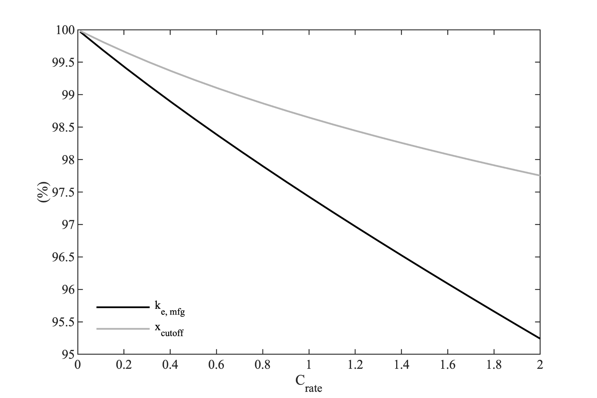
The premature cutoff effect mentioned earlier is illustrated by the grey curve in this figure. This effect is neglected by the simple approximation provided by the prior equation.
The manufacturer’s rated discharge knockdown factor as calculated by numerical integration is given by the black curve in this figure. For our power cell, this effect is small, but worth computing - for an energy cell, this effect can likely be neglected.
$$k_{e,mfg}=0.9743$$Pack Mass Overhead
As installed in an aircraft, battery packs contain more than just cells. Everything in a pack that is not a cell contributes to the pack mass overhead. This will include provisions for current collection, pack structure, thermal protection and management, the BMS, etc.
The pack mass knockdown factor is simply the total cell mass (number of cells times the mass of a single cell) divided by the battery pack mass.
$$k_{m}=\,\frac{N_{c}\,m_{c}}{m_{b}}$$Exactly what is book-kept as pack mass vs. airframe mass can get a bit messy. If an aircraft has a removable pack, I would suggest starting by considering everything that comes off when a pack is removed is the pack mass - and everything left behind is part of the airframe. These details do not matter for this discussion - every pack will have some overhead mass.
The pack mass overhead is likely one of the most familiar contributions to the knockdown factor. Many discussions center around whether a battery specific energy level is specified at the cell level or the pack level - the pack mass overhead is exactly this difference. Practitioners often think and communicate in terms of pack ‘overhead’ - more formally called the ‘pack non-cell mass fraction’. Advanced packs have an overhead of about 15-20%.
Our knockdown factor calculation works in terms of the ‘pack cell mass fraction’ - which is calculated as one minus the overhead. Advanced packs will have a pack cell mass fraction of about 80-85%. For our example, we will assume a pack with 18% overhead.
$$k_{m}=0.82$$Cell Energy Knockdown Factor
We now have all the parts required to assemble our cell energy knockdown factor. Each contribution represents an independent effect referenced to the absolute reference energy (except for the mass contribution) and so they can be combined by multiplying them together - except for the manufacturer’s rated discharge knockdown factor, which must appear in the denominator.
$$k=\,\frac{k_{m}\,k_{e,DOD}\,k_{e,FR\&R}\,k_{Q}}{k_{e,mfg}\,}$$Plugging in the five terms calculated for the example case over the past few articles gives us a combined knockdown factor of 0.532.
$$k=\,\frac{\left(0.82\right)\,\left(0.763\right)\,\left(0.92\right)\,\left(0.9\right)}{0.9743\,}=0.532$$For our example cell, the manufacturer’s rated specific energy is 230 Wh/kg - but in this installation, the aircraft achieves a pack specific energy of 122 Wh/kg.
Our example mission required 3250 hp-m of energy from the battery - which is a bit over 40 kWh. Our aircraft would need a 330 kg (727 lb) pack.
Without the context provided by the vehicle mass and the reasonableness of the hover and cruise powers, this doesn’t mean a whole lot. That is on purpose. I leave those things out because the focus here should not be on the merits of the example vehicle, but instead on how these calculations can be performed for any candidate vehicle.
Our knockdown factor provides a straightforward way to size a battery pack for an electric aircraft. It includes effects of pack mass overhead, restricted depth of discharge for power limits and a variety of operational considerations, cell finite rate efficiency (including resistance growth at EOL), and capacity fade at EOL.
Better than a black-box calculation of all these effects, the knockdown factor buildup approach provides transparency into each effect and its relative contribution to the pack size. Hopefully you have also gained some intuition as to what factors influence each contribution and what you might do as a designer to effect change.
Although it has not been a focus of this discussion, I hope it is apparent how much of an effect conops and mission requirements have on these calculations. A small UAS may have minimal pack overhead and could use a larger fraction of the cell capacity. EOL considerations may not matter - allowing the vehicle performance to fade as the cells age. This situation will result in a very different knockdown factor and realized battery specific energy. These are decisions that are subject to trade.
Conclusion
This series was motivated by the differences between liquid fuel and batteries for aircraft propulsion. While it may seem like we have lost track of that motivation, I hope that is not the case. Every pound of liquid fuel contains the same energy - it does not matter which part of the tank it comes out of, how old the tank is, or how fast you burn it. Put another way, the specific energy knockdown factor for liquid fuel is 1.0.
Responsible conceptual designers of battery electric aircraft need to understand these effects and quantify them in their sizing calculations. Failure to do so will result in aircraft that fail to meet design expectations.
Although this is a good place to stop this series of articles, there is much more to be considered when designing an electric aircraft. Perhaps there will be another article series down the road. If you think that is a good idea, leave a comment and let me know what you would like to see covered.